16S Microbiome Analysis in Qiita

Analysis of Closed Reference processing

To create an analysis, select Create new analysis from the top menu.

This will take you to a list of studies with samples available to you for analysis, divided between your studies and publically available (‘Other’) studies.

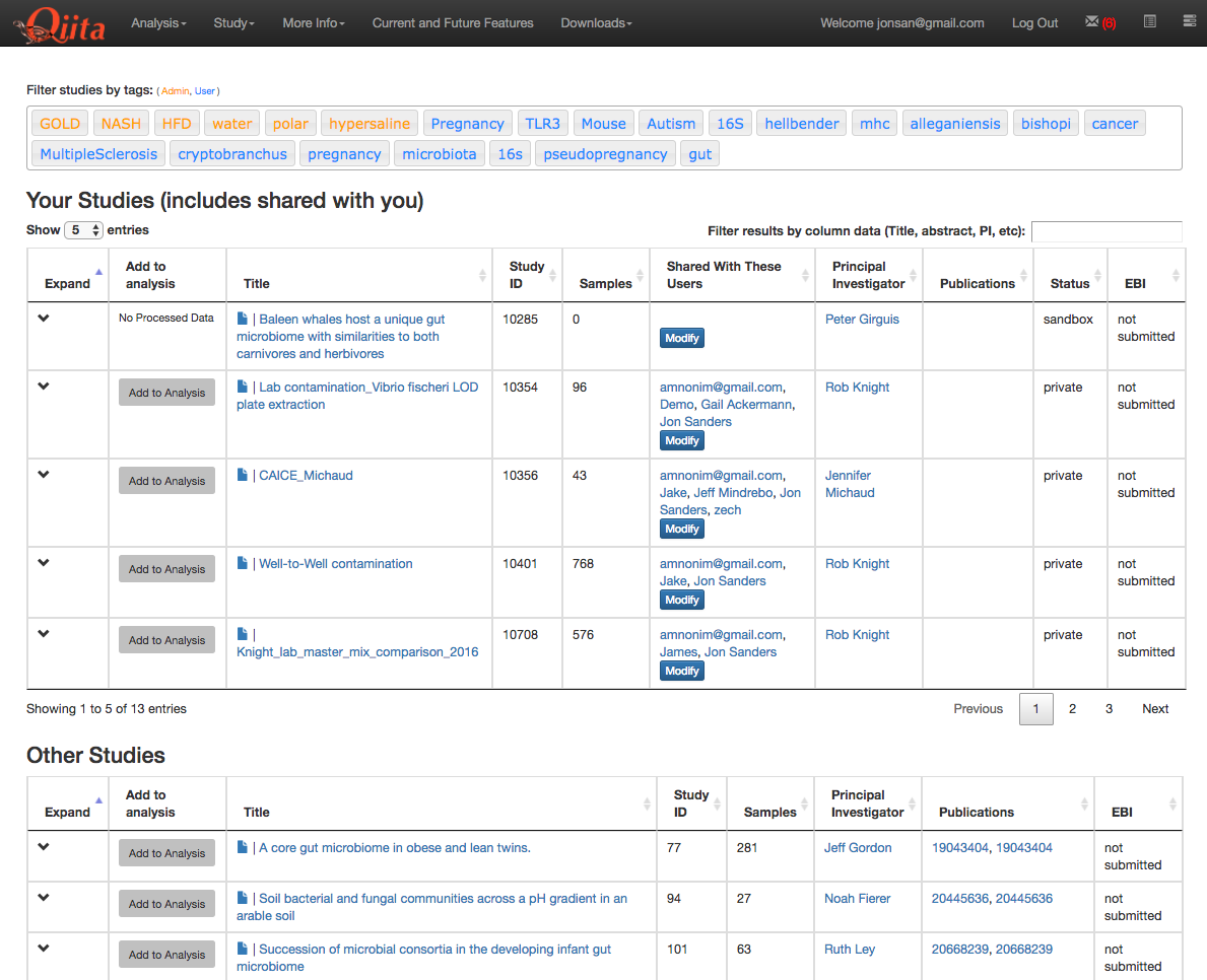
Find the study you created for this tutorial under “Your Studies”. Click the down arrow at the left of the row. This will expand the study to expose all the objects from that study that are available to you for analysis.

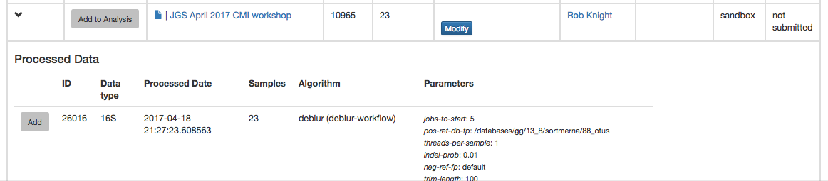
You could add all of these objects to the analysis by selecting the Add to Analysis button. We will just add the Closed Reference OTU table object by clicking Add in that row.

Now, the second-right-most icon at the top bar should be green, indicating that there are samples selected for analysis.

Clicking on the icon will take you to a page where you can refine the samples you want to include in your analysis. Here, all 23 of our samples are currently included:

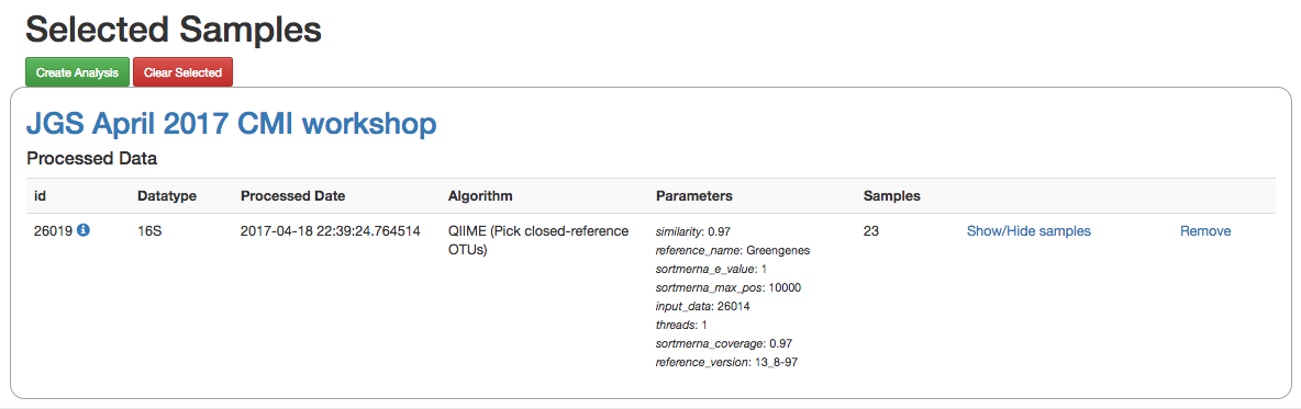
You could optionally exclude particular samples from this set by clicking on “Show/Hide samples”, which will show each individual sample name along with a “remove” option. (Removing them here will mask them from the analysis, but will not affect the underlying files an any way.)

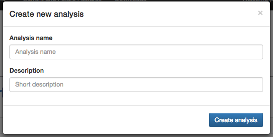
This should be good for now. Click the “Create Analysis” button, enter a name and description, then click “Create analysis”.

This brings you to the analysis commands selection page, where you can specify the steps in your analysis.

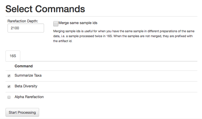
For this analysis, let’s go ahead and select the commands Summarize Taxa and Beta Diversity (Alpha Rarefaction can take some time to run).

We will also need to specify an even sampling or rarefaction depth. All the samples in the analysis will be randomly subsampled to this number of sequences, reducing potential biases. Samples with fewer than this number of sequences will be excluded, which can also be useful for excluding things like blanks.

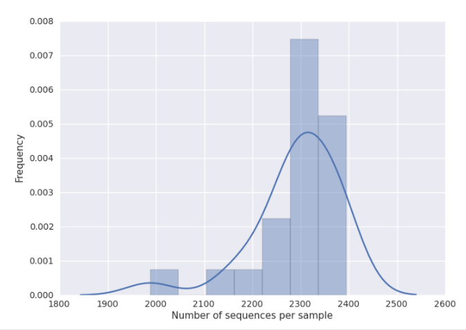
You can get a good idea of where to set this threshold by looking at the histogram generated by summarizing the input closed-reference OTU table, as discussed in 16S Microbiome Analysis in Qiita. Here, it looks like 2100 would be an appropriate cutoff: it excludes one clear outlier, but retains most of the samples.

Enter 2100 in the rarefaction depth field, select the check boxes for Summarize Taxa and Beta Diversity, and click “Start Processing”. You will see a list each step in the analysis, followed by its status:

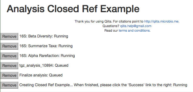
When the analysis is finished, click the ‘Success’ link to see the results.

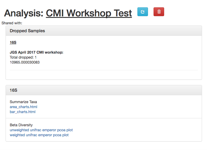
The results page will have sections indication which samples were dropped due to insufficient numbers of reads, as well as sections for each data type.

Here, we have taxonomy summaries and beta diversity PCoA plots available.

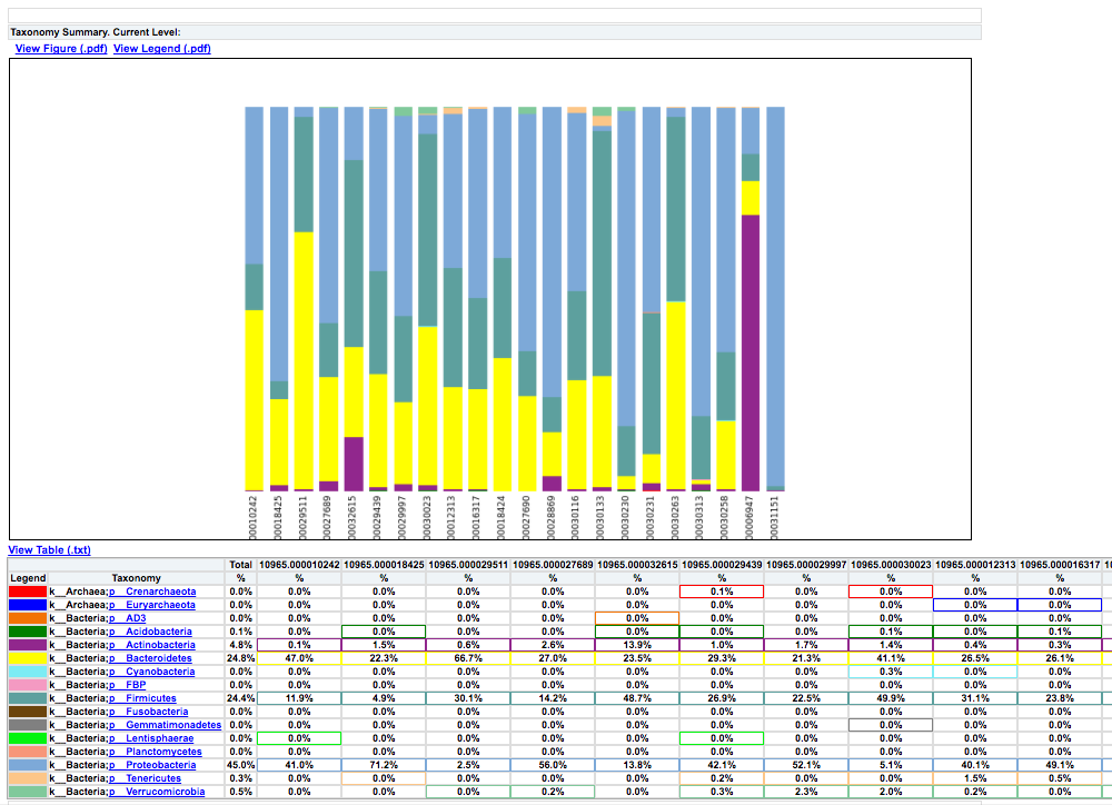
Clicking on bar_charts.html under “Summarize Taxa” will take you to a visualization of the taxa that were found in your sample:

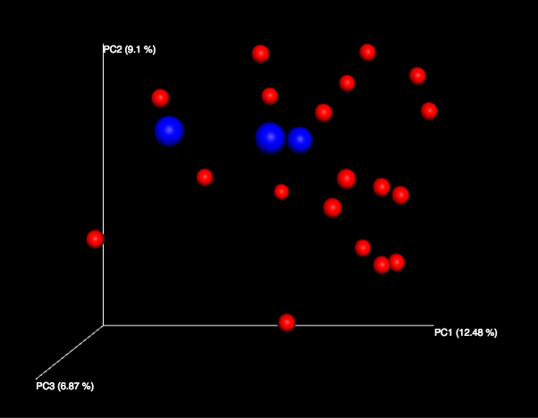
Under “Beta Diversity”, you will have a selection of Principle Coordinates Analyses of different measures of beta diversity, or the similarity between samples.

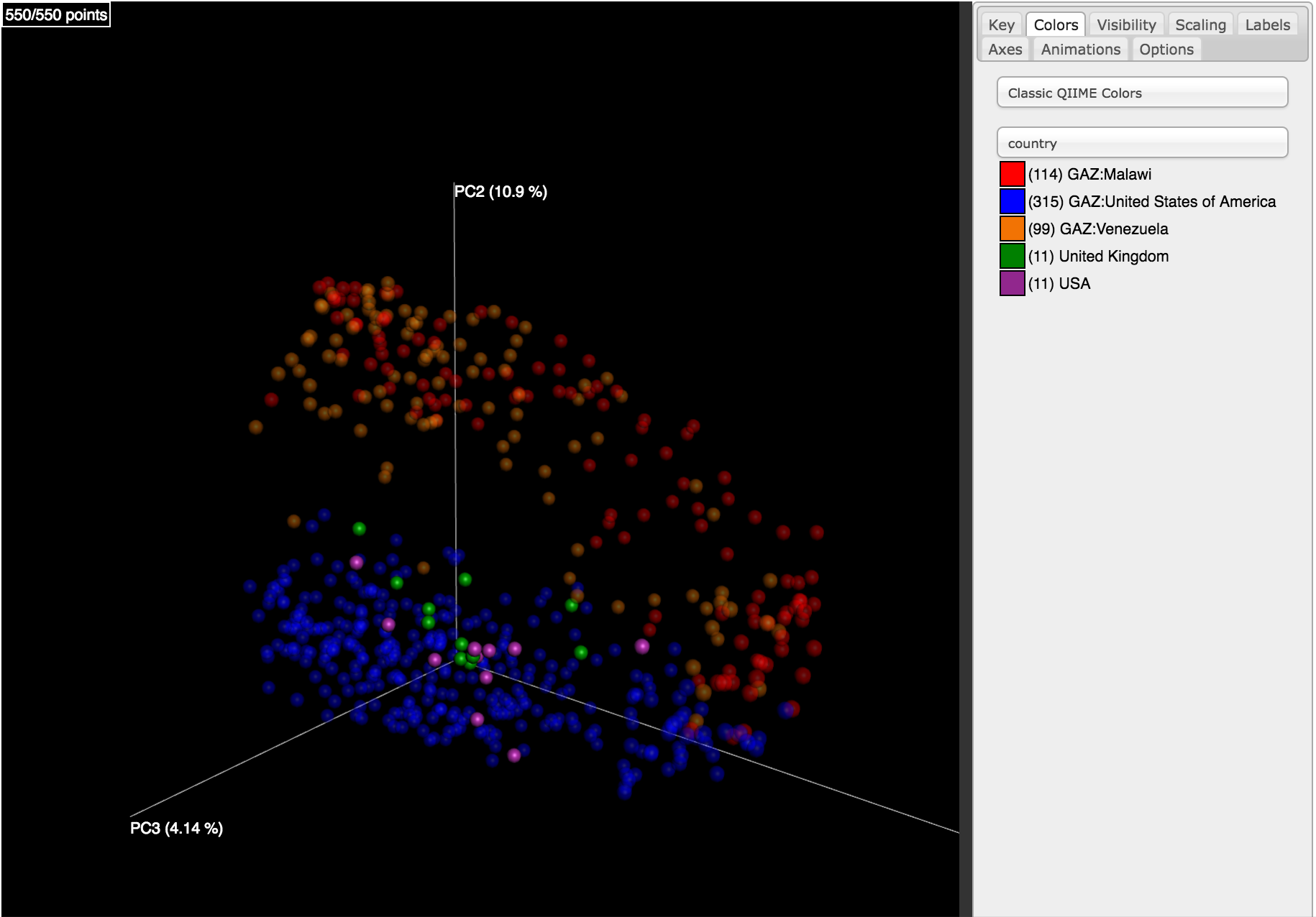
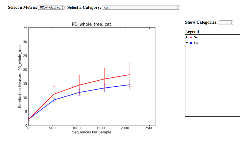
Clicking on one (say, unweighted unifrac emperor pcoa plot) will open an interactive visualization of the similarity among your samples. Generally speaking, the more similar the samples, the closer the are likely to be in the PCoA ordination. The Emperor visualization program offers a very useful way to explore how patterns of similarity in your data associate with different metadata categories. Here, I’ve colored the points in our test data by cat ownership.

Let’s take a few minutes now to explore the various features of Emperor. Open a new browser window with the Emperor tutorial and follow along with your test data.

Finally, if you ran Alpha Rarefaction, you will also have a link to interactive plots that can be used to show how different measures of alpha diversity correlate with different metadata categories:

Analysis of deblur processing

Creating an analysis of your deblurred data is virtually the same as the process for the Closed Reference data, but there are a few quirks.

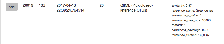
First, because the deblur process creates two separate BIOM tables, you’ll want to make a note of the specific object ID number for the artifact you want to use. In my case, that’s ID 26017, the deblurred table with ‘only-16s’ reads.

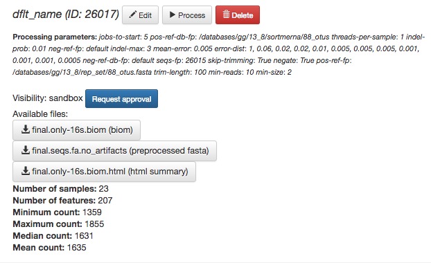
The specific ID for your table will be unique, so make a note of it, and you can use it to select the correct table for analysis.

Second, currently only the Beta Diversity analysis command option is working with deblurred data.

Creating a meta-analysis

One of the most powerful aspects of Qiita is the ability to compare your data with hundreds of thousands of samples from across the planet. Right now, there are almost 130,000 samples publicly available for you to explore:

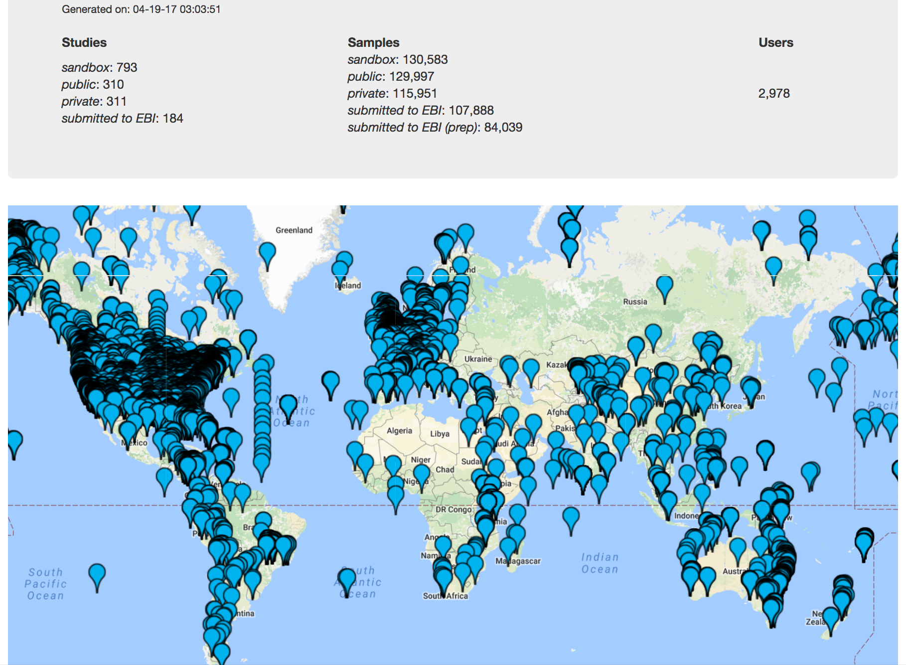
(You can get up-to-date statistics by clicking “Stats” under the “More Info” option on the top bar.)

Creating a meta-analysis is just like creating an analysis, except you choose data objects from multiple studies. Let’s start creating a meta-anlysis by adding our Closed Reference OTU table to a new analysis.

Next, we’ll look for some additional data to compare against.

You noticed the ‘Other Studies’ table below ‘Your Studies’ when adding data to the analysis. (Sometimes this takes a while to load - give it a few minutes.) These are publicly available data for you to explore, and each should have processed data suitable for comparison to your own.

There are a couple tools provided to help you find useful public studies.

First, there are a series of “tags” listed at the top of the window:

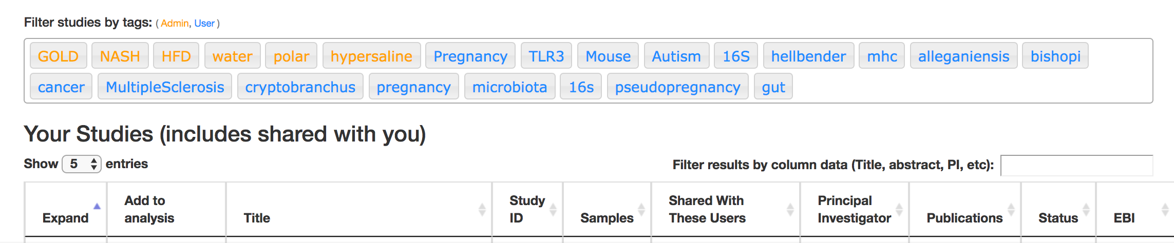
There are two types of tags: admin-assigned (yellow), and user-assigned (blue). You can tag your own study with any tag you’d like, to help other users find your data. For some studies, Qiita administrators will apply specific reserved tags to help identify particularly relevant data. The “GOLD” tag, for example, identifies a small set of highly-curated, very well-explored studies. If you click on one of these tags, all studies not associated with that tag will disappear from the tables.

Second, there is a search field that allows you to filter studies in real time. Try typing in the name of a known PI, or a particular study organism – the thousands of publicly available studies will be filtered down to something that is easier to look through.

Let’s try comparing our data to the “Global Gut” dataset of human microbiomes from the US, Africa, and South America from the study “Human gut microbiome viewed across age and geography” by Yatsunenko et al. We can search for this dataset using the DOI from the paper: 10.1038/nature11053.

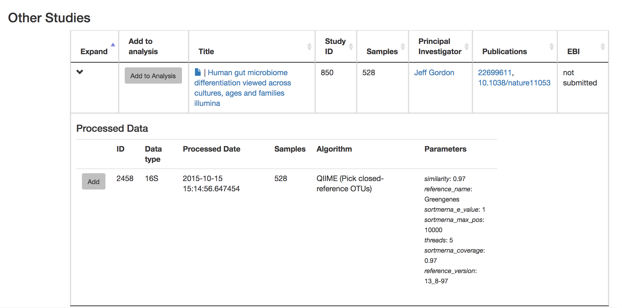
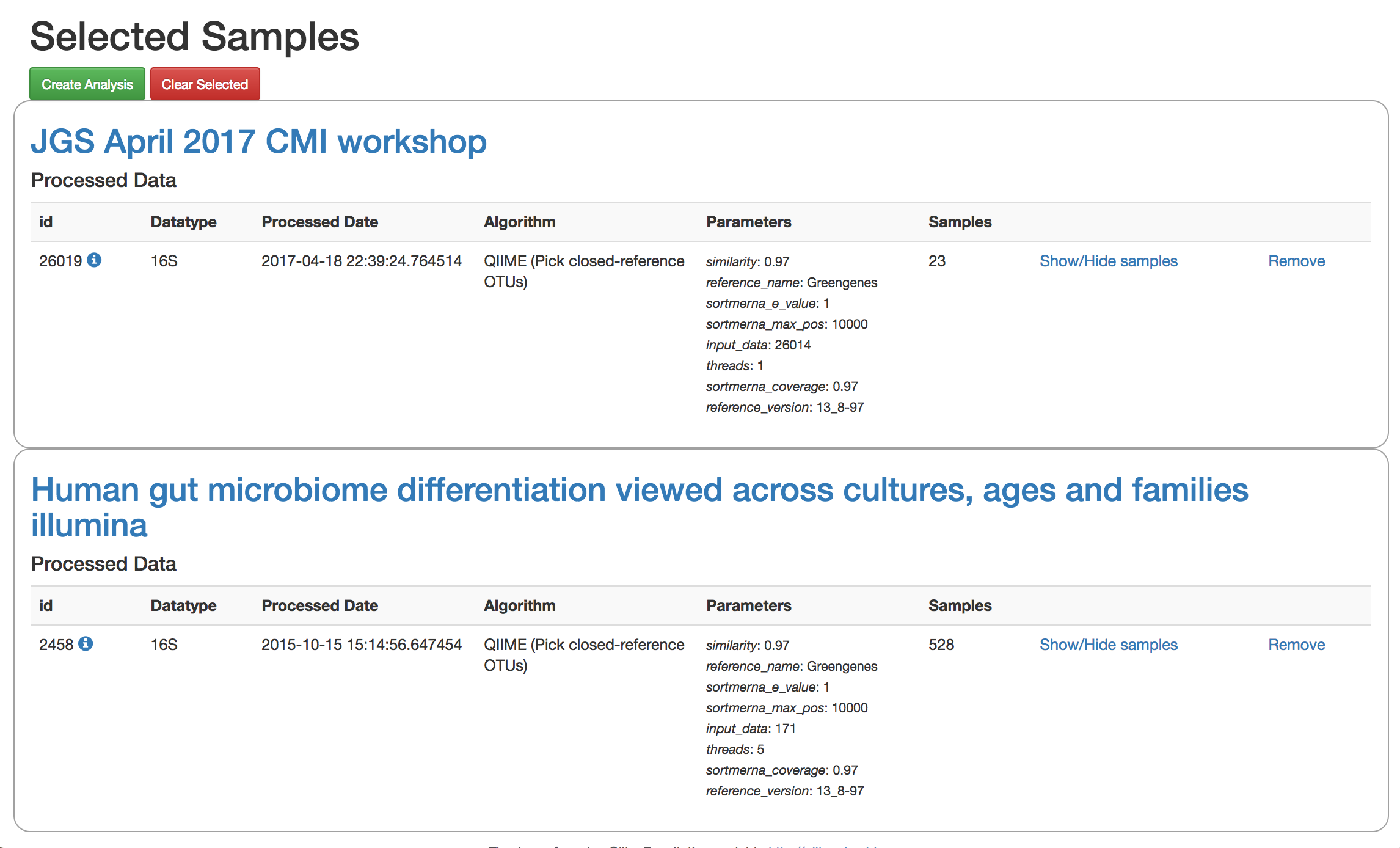
Add the closed reference OTU table from this study to your analysis. You should now be able to click the green analysis icon in the upper right and see both your own OTU table and the public study OTU table in your analysis staging area:

You can now click “Create Analysis” just as before to begin specifying analysis steps. This time, let’s just do the beta diversity step. Select the Beta Diversity command, enter a rarefaction depth of 2100, and click “Start Processing”.

Because you’ve now expanded the number of samples in your analysis by more than an order of magnitude, this step will take a little longer to complete. But when it does, you will be able to use Emperor to explore the samples in your test dataset to samples from around the world!