Now, we’ll upload some actual microbiome data to explore. To do this, we need to add the data themselves, along with some information telling Qiita about how those data were generated.
Adding a preparation template and linking it to raw data
Where the sample info file has the biological metadata associated with your samples, the preparation info file contains information about the specific technical steps taken to go from sample to data. Just as you might use multiple data-generation methods to get data from a single sample – for example, target gene sequencing and shotgun metagenomics – you can have multiple prep info files in a single study, associating your samples with each of these data types. You can learn more about prep info files at the Qiita documentation.
Go back to the “Upload Files” interface. In the example data, find and upload the 3 “.fastq.gz files” and the “prep_info_16S.txt” file.
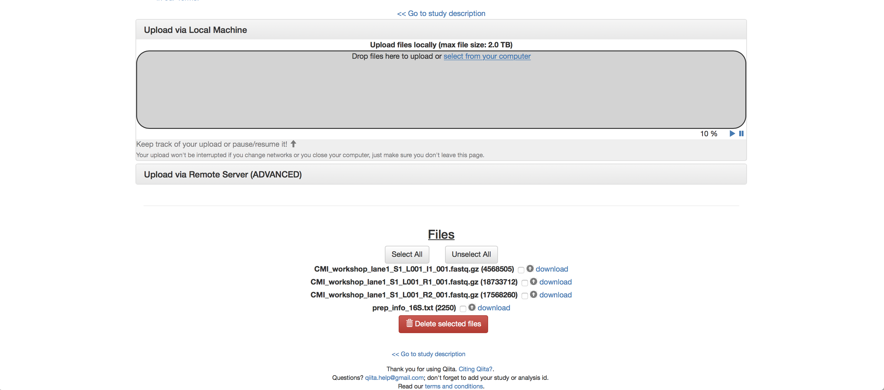
These files will appear under “Files” when they finish uploading.
Then, go to the study description. Now you can click the “Add New Preparation” button. This will bring up the following dialogue:
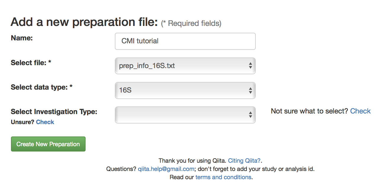
Select “prep_info_16S.txt” from the “Select file” dropdown, and “16S” as the data type. Optionally, you can also select one of a number of investigation types that can be used to associate your data with other like studies in the database. Click “Create New Preparation”.
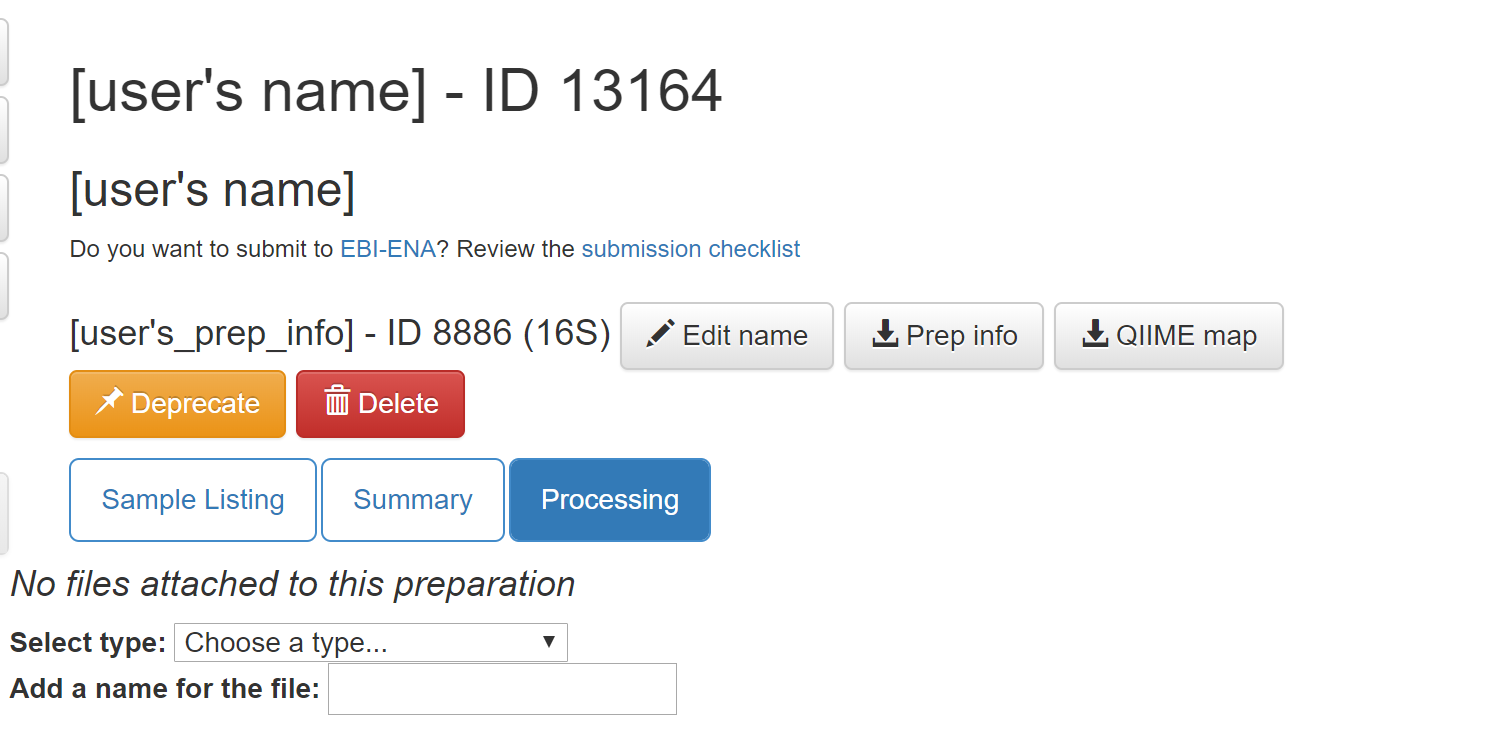
You should now be brought to a “Processing” tab of your preparation info:
By clicking on the “Summary” tab on this page you can see the preparation info that you uploaded.
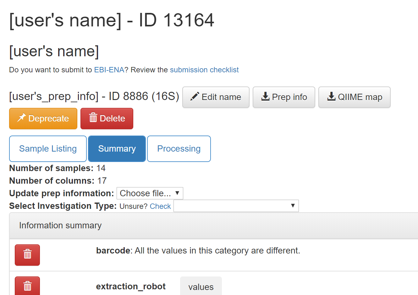
As the owner of the study, you will also have the options to delete or deprecate the preparation. Once an analysis has been created from any object in a preparation, you will be unable to delete the prep. Deprecating the preparation lets others know it is an older version.
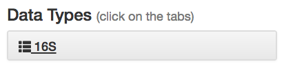
In addition, you should see a “16S” button appear under “Data Types” on the menu to left:
You can click this to reveal the individual prep info files of that data type that have been associated with this study:
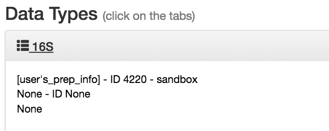
If you have multiple 16S preparations (for example, if you sequenced using several different primer sets), these would each show up as a separate entry here.
Now, you can associate the sequence data from your study with this preparation.
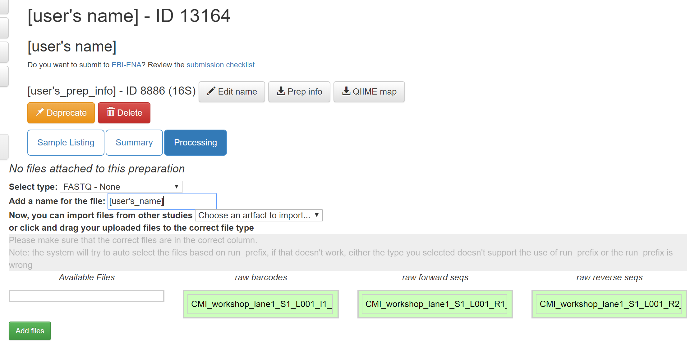
Select the processing tab again. In the prep info dialogue, there is a dropdown menu below the words No files attached to this preparation, labeled “Select type”. Click “Choose a type” to see a list of available file types. In our case, we’ve uploaded FASTQ-formatted files for all samples in our study, so we will choose “FASTQ - None”. In some cases outside of this tutorial, you may have per sample FASTQ files, so take care in considering which data type you are handling.
Magically, this will prompt Qiita to associate your uploaded files with the corresponding samples in your preparation info. (Our prep info file has a column named run_prefix, which associated the sample_name with the file name prefix for that particular sample).
You should see this as filenames showing up in the green: raw barcodes (file with I1 in its name), raw forward seqs (R1 in name) and raw reverse seqs (R2 in name) columns below the import dropdown. You’ll want to give the set of these FASTQ files a name (Add a name for the file field below Select type: FASTQ - None), and then click “Add files” below.
That’s it! Your data are ready for processing.
Exploring the raw data
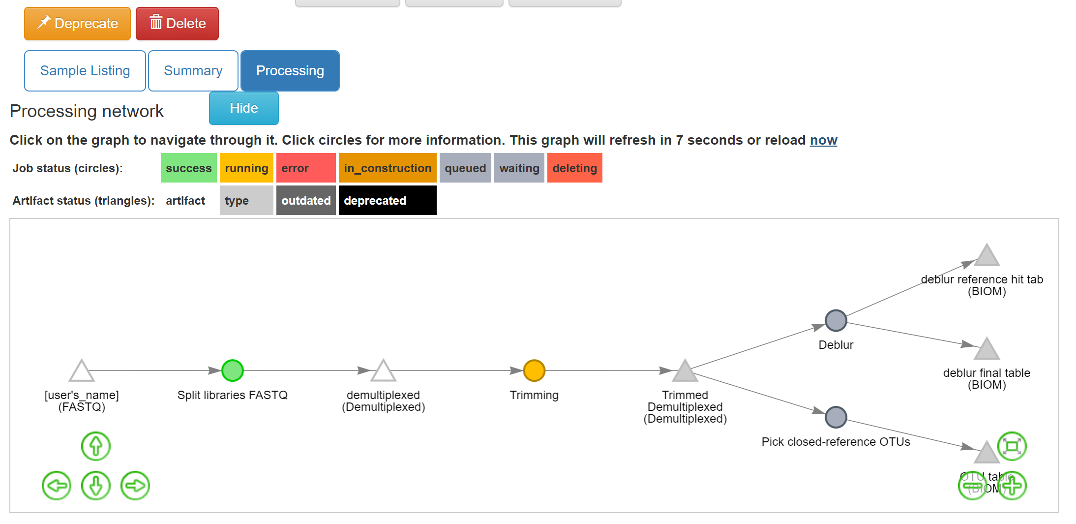
Click on the 16S menu on the left. Now that you’ve associated sequence files with this prep, you’ll have a “Processing network” displayed:
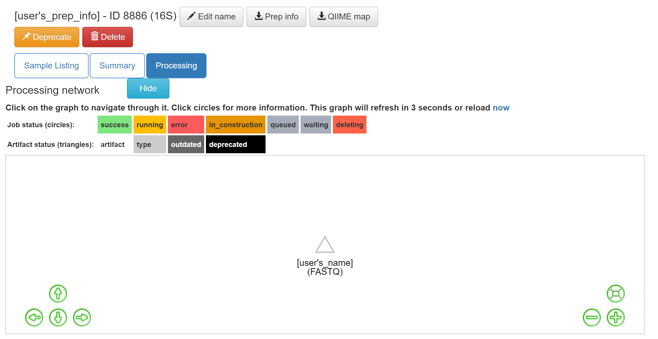
If you see this message:

It means that your files need time to load. Refresh your screen after about 1 minute.
Your collection of FASTQ files for this prep are all represented by a single object in this network, called “[user’s_name] (FASTQ)” in the example. Click on the object.
Now, you’ll have a series of choices for interacting with this object. You can click “Edit” to rename the object, “Process” to perform analyses, or “Delete” to delete it. In addition, you’ll see a list of the actual files associated with this object.
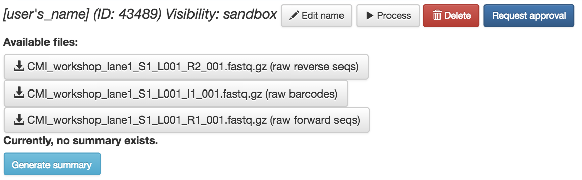
Scroll to the bottom, and you’ll also see an option to generate a summary of the object.

If you click this button, it will be replaced with a notification that the summary generation has been added to the processing queue.
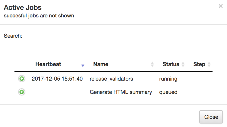
To check on the status of the processing job, you can click the rightmost icon at the top of the screen:

This will open a dialogue that gives you information about currently running jobs, as well as jobs that failed with some sort of error. Please note, this dialogue keeps the entire history of errors that Qiita encountered for your jobs, so take notice of dates and times in the Heartbeat column.
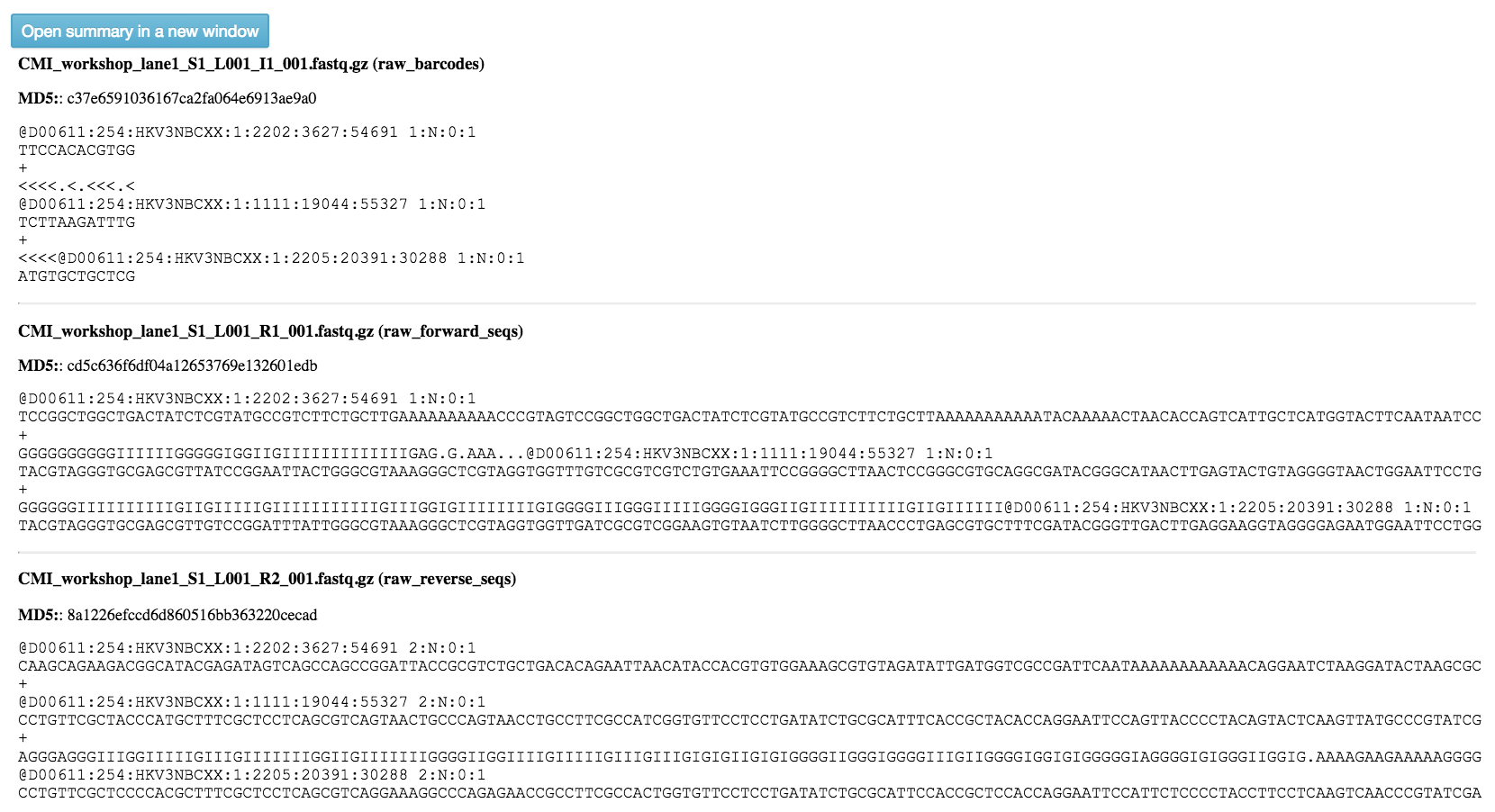
The summary generation shouldn’t take too long. You may need to refresh your screen. When it completes, you can click back on the FASTQ object and scroll to the bottom of the page to see a short peek at the data in each of the FASTQ files in the object. These summaries can be useful for troubleshooting.
Now, we’ll process the raw data into something more interesting.
Processing 16S data
Scroll back up and click on the “CMI tutorial - 14 skin samples(FASTQ)” artifact, and select “Process”. Below the files network, you will now see a “Choose command” dropdown menu. Based on the type of object, this dropdown menu will give a you a list of available processing steps.
For 16S “FASTQ” objects, the only available command is “Split libraries FASTQ”. The converts the raw FASTQ data into the file format used by Qiita for further analysis (you can read more extensively about this file type here).
Select the “Split libraries FASTQ” step. Now, you will be able to select the specific combination of parameters to use for this step in the “Choose parameter set” dropdown menu.
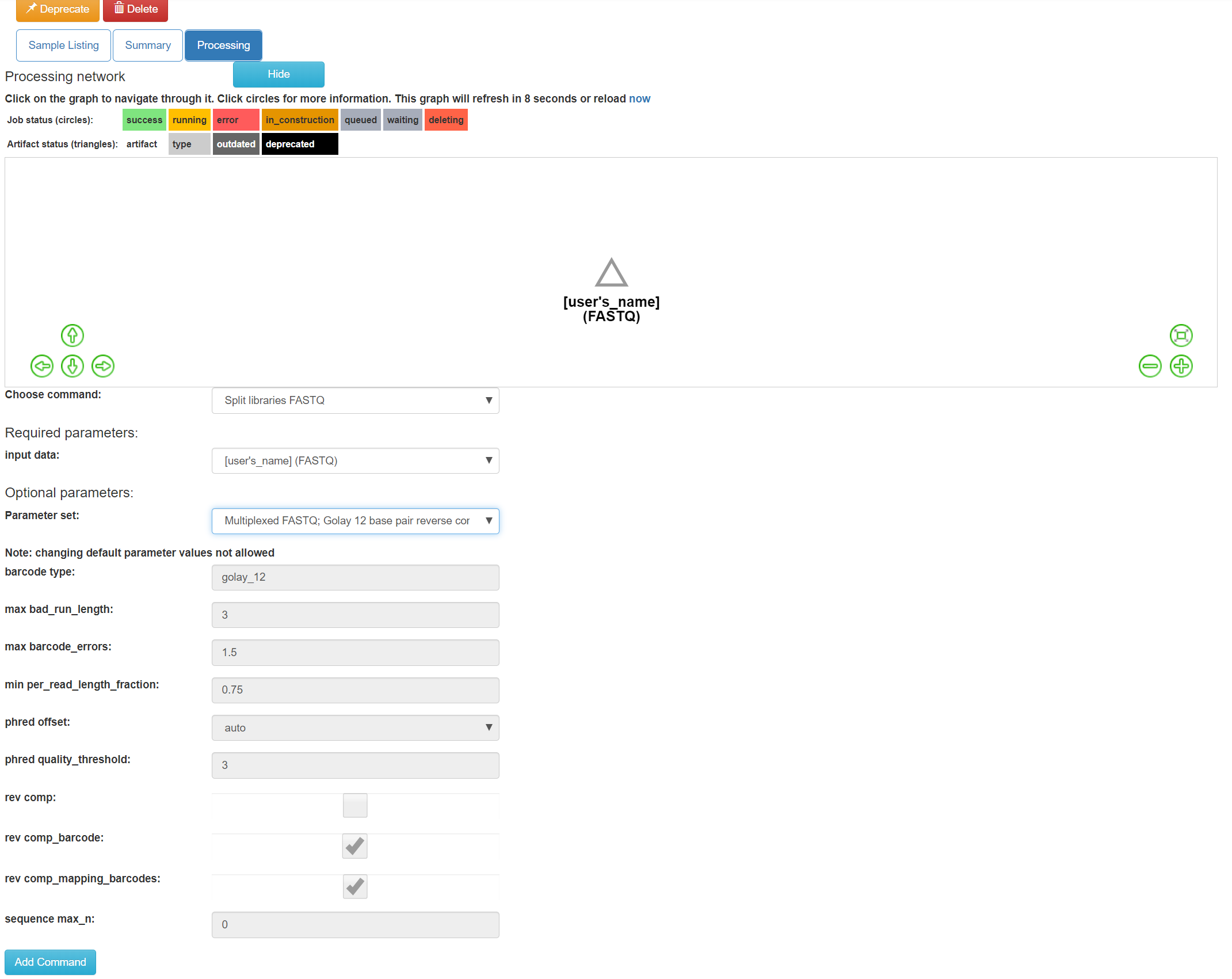
For our files, choose “Multiplexed FASTQ; Golay 12 base pair reverse complement mapping file barcodes with reverse complement barcodes”. The specific parameter values used will be displayed below. For most raw data coming out of the Knight Lab you will use the same setting.
Click “Add Command”.
You’ll see the files network update. In addition to the original white object, you should now see the processing command (represented in yellow) and the object that will be produced from that command (represented in grey).
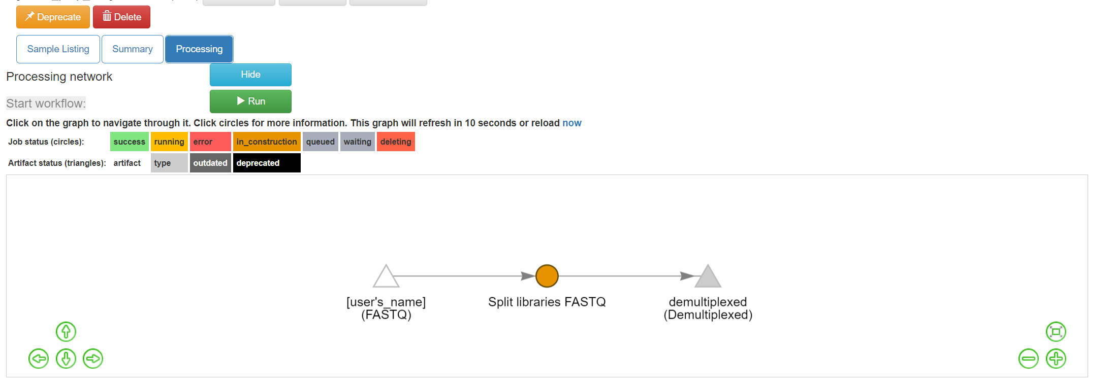
You can click on the command to see the parameters used, or on an object to perform additional steps.
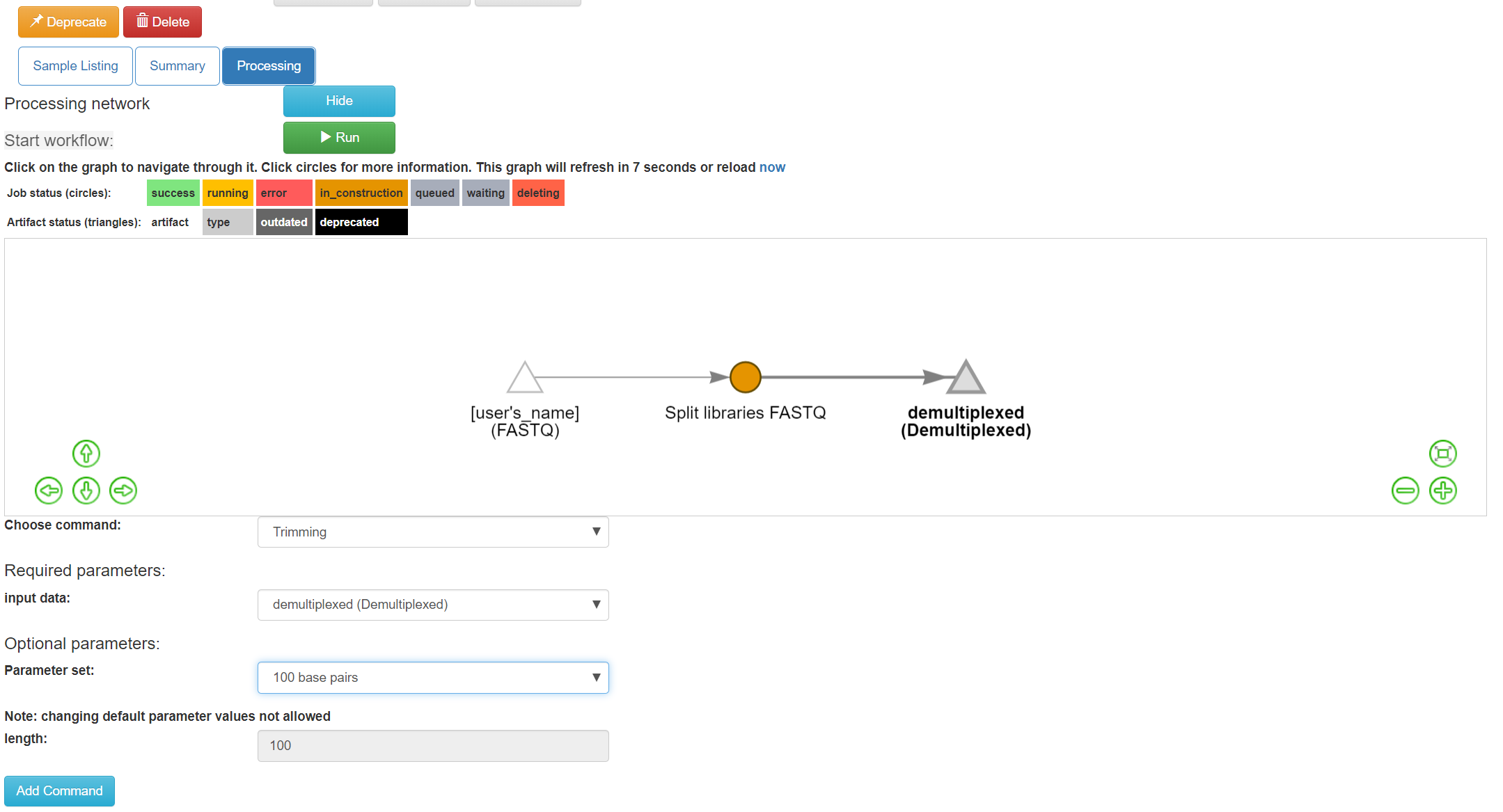
Next we want to trim to a particular length, to ensure our samples will be comparable to other samples already in the database. Click back on the “demultiplexed (Demultiplexed)”. This time, select the Trimming operation. Currently, there are seven trimming length options. Let’s choose “100 basepairs”, which trims to the first 100bp, for this run, and click “Add Command”.
Click “Add Command”, and you will see the network update:
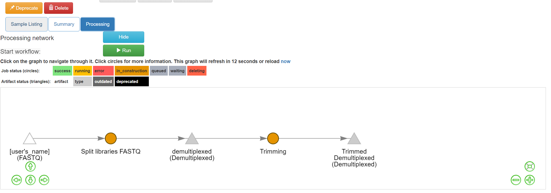
Note that the commands haven’t actually been run yet! (We’ll still need to click “Run” at the top.) This allows us to add multiple processing steps to our study and then run them all together.
We’re going to process our sequence files using two different workflows. In the first, we’ll use a conventional reference-based OTU picking strategy to cluster our 16S sequences into OTUs. This approach matches each sequence to a reference database, ignoring sequences that don’t match the reference. In the second, we will use deblur, which uses an algorithm to remove sequence errors, allowing us to work with unique sequences instead of clustering into OTUs. Both of these approaches work great with Qiita, because we can compare the observations between studies without having to do any sort of re-clustering!
The closed-reference workflow
To do closed reference OTU picking, click on the “Trimmed Demultiplexed (Demultiplexed)” object and select the “Pick closed-reference OTUs” command. We will use the “Defaults” parameter set for our data, which are relatively small. For a larger data set, we might want to use the “Defaults - parallel” implementation.
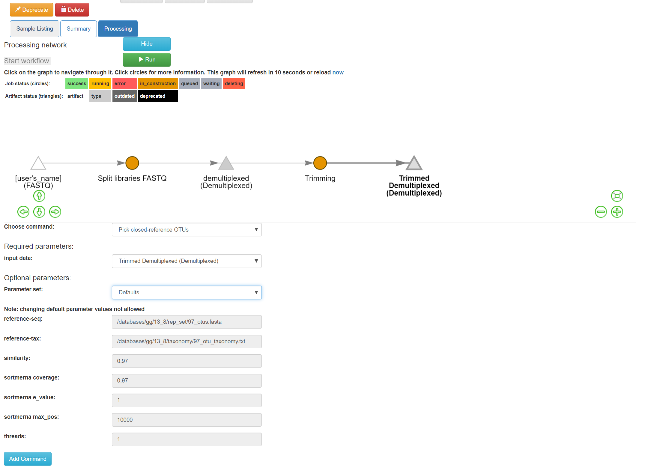
By default, Qiita uses the GreenGenes 16S reference database. You can also choose to use the Silva 119 18S databsase, or the UNITE 7 fungal ITS database.
Click “Add Command”, and you will see the network update:
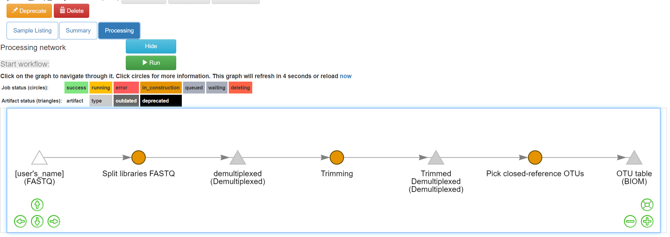
Here you can see the blue “Pick closed-reference OTUs” command added, and that the product of the command is a BIOM-formatted OTU table.
That’s it!
The deblur workflow
The deblur workflow is only marginally more complex. Although you can deblur the demultiplexed sequences directly, “deblur” works best when all the sequences are the same length. By trimming to a particular length, we can also ensure our samples will be comparable to other samples already in the database.
Click back on the “Trimmed Demultiplexed (Demultiplexed)” object. This time, select the Deblur operation. Choose “Deblur” from the “Choose command” dropdown, and “Defaults” for the parameter set.
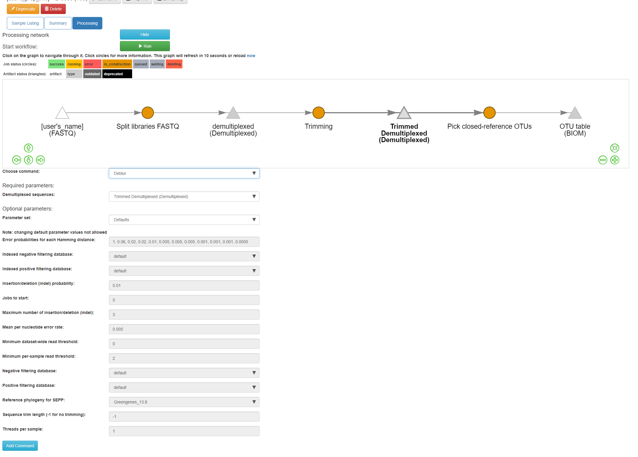
Add this command to create this workflow:
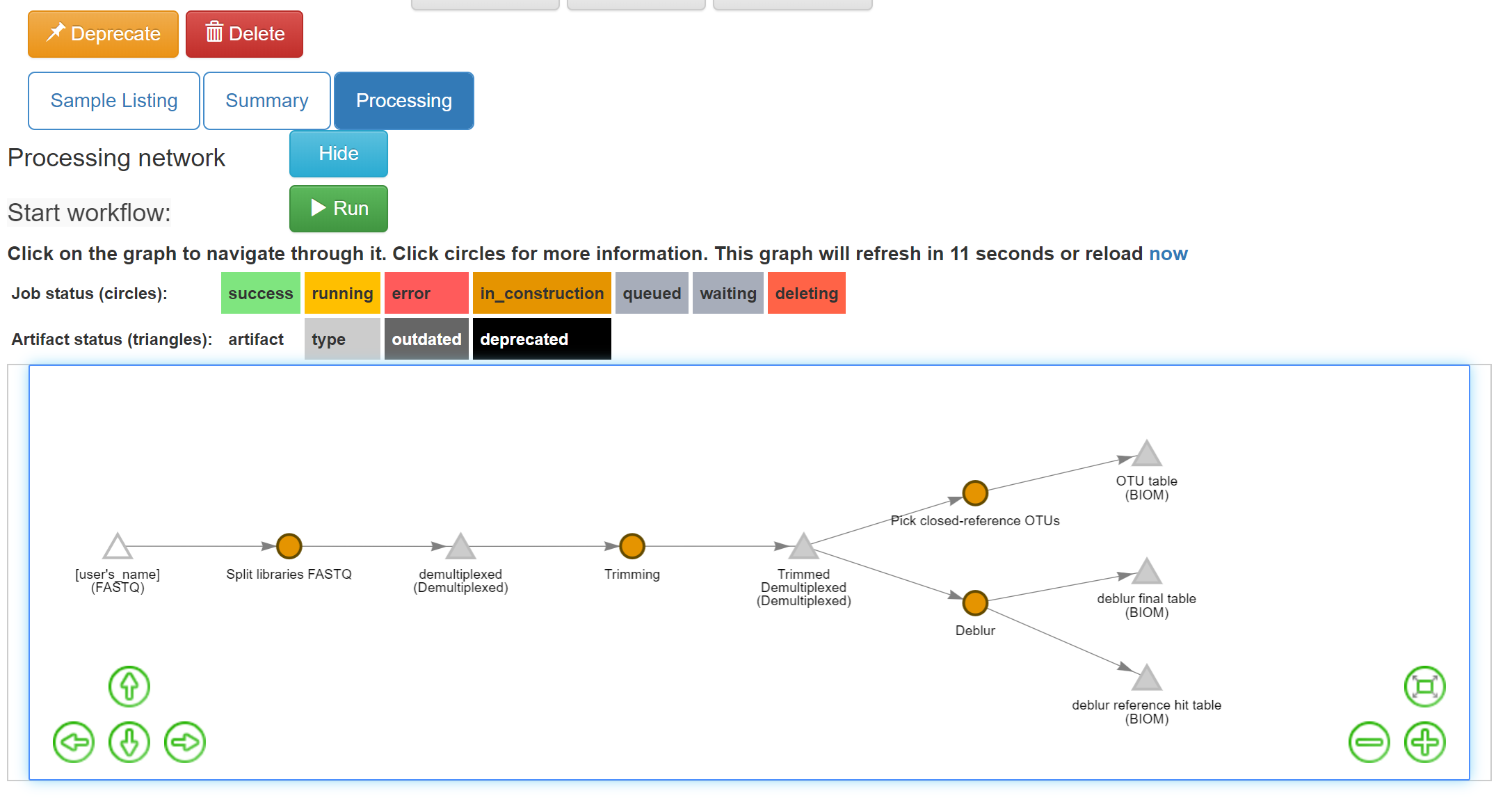
Now you can see that we have the same “Trimmed Demultiplexed (Demultiplexed)” object being used for two separate processing steps – closed-reference OTU picking, and deblur.
As you can see, “deblur” produces two BIOM-formatted OTU tables as output. The “deblur reference hit table (BIOM)” contains deblurred sequences that have been filtered to try and exclude things like organellar mitochondrial reads, while “deblur final table (BIOM)” has all the sequences.
Running the workflow
Now, we can see the whole set of commands and their output files:
Click “Run” at the top of the screen, and Qiita will start executing all of these jobs. You’ll see a “Workflow submitted” banner at the top of your window.
The full workflow can take time to load depending on the amount of samples and Qiita workload. You can keep track of what is running by looking at the colors of the command artifacts. If yellow, the commands are being run now. If green, the commands have successfully been run. If red, the commands have failed.
Once objects have been generated, you can generate summaries for them just as you did for the original “FASTQ” object.
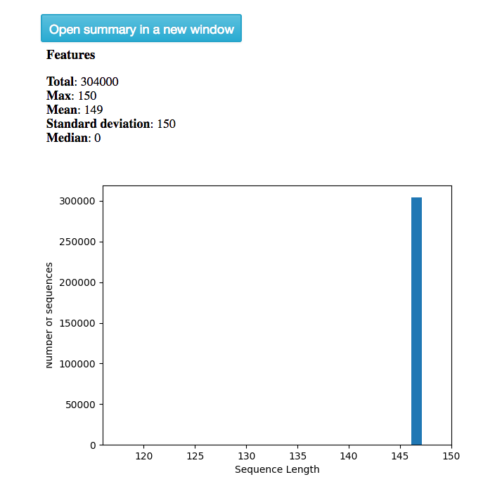
The summary for the “demultiplexed (Demultiplexed)” object gives you information about the length of sequences in the object:
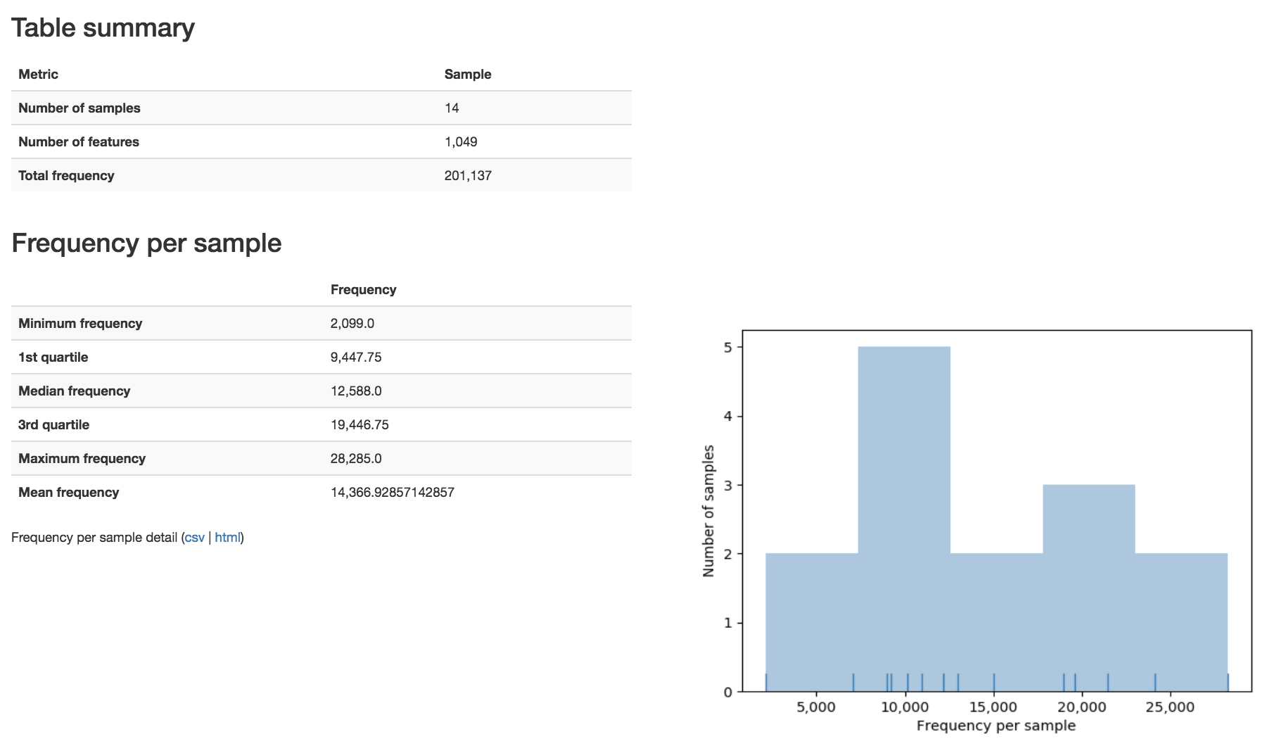
The summary for a BIOM-format OTU table gives you a table summary, details regarding the frequency per sample, and a histogram of the number of features per sample: